One of the casualties of the forthcoming changes to the A-Level syllabus is the Decision Maths module(s). The “standard” A (and AS) Level will consist of Pure Maths and a combined applied maths paper, made up of content from both Mechanics and Statistics.
I’m not sure how I feel about this – on the one hand, Decision 1 contains some really interesting maths: want to know how your SatNav determines your route? Decision 1 has the answer. Want to know how Excel sorts data? D1 explores the Bubble Sort and Shuttle Sort algorithms, as well as explaining how to determine the efficiency of an algorithm. Plus I make a cameo appearance in the EdExcel D1 text book – my 15 minutes of fame!
But answering some (many) of the exam questions can become a little tedious, with the student forced to replicate the steps taken by a computer to use an algorithm to solve a problem.
But regardless of the above, I was delighted to discover a new application of the Traveling Salesman Problem that we study in the course.
The Traveling Salesman Problem (or TSP for short) is simple in principle, but soon escalates to become very calculation heavy.
A salesman needs to visit all the towns in his area, before returning home from where he started. In achieving his goal he wants to travel as short a distance as possible and the solution to the TSP is this route.
Imagine he only has 3 towns to visit – he has 3 choices for his first town, then 2 for his second, and only 1 for his third, so there are 3x2x1 = 6 possible solutions, although we can halve this as the length of the route ABC will be the same as CBA.
Add a fourth town and there are ½ of 4x3x2x1 = 12 different routes, five towns gives ½ of 5x4x3x2x1 = 60 – the numbers soon start getting very big and even a computer would begin to struggle to compute all the various different permutations to find the shortest route.
So we use an algorithm – in fact we use two. Its such a difficult problem that we don’t necessarily find the optimal solution. We use the “Nearest Neighbour” algorithm to find the upper bound – a distance we know that can contain a route, and then we use the Lower Bound algorithm to find the shortest what the optimal route could be. We now have a range of values between which the optimal solution must lie. If the range is small we may be happy to go with our upper bound route, if not we can try the tour improvement algorithm.
Rather than try to explain these algorithms, this short video offers a good insight into how they work.
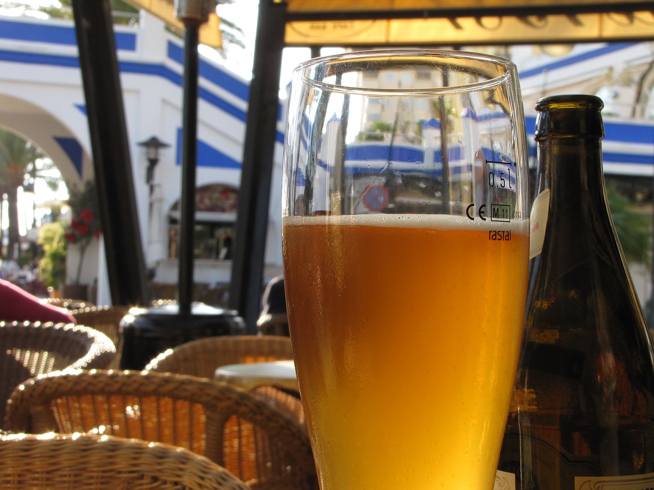
“But you promised me a pint!” I hear you cry. “Whats all this got to do with the price of beer?”
I’m getting to that now.
Earlier this week, I stumbled on a superb piece of mathematics that found the shortest route that would take in all 24,727 (yes – twenty four thousand, seven hundred and twenty seven) pubs in the UK.
You can read all about it here …
… or you can just enjoy the majesty of the map that shows the route:
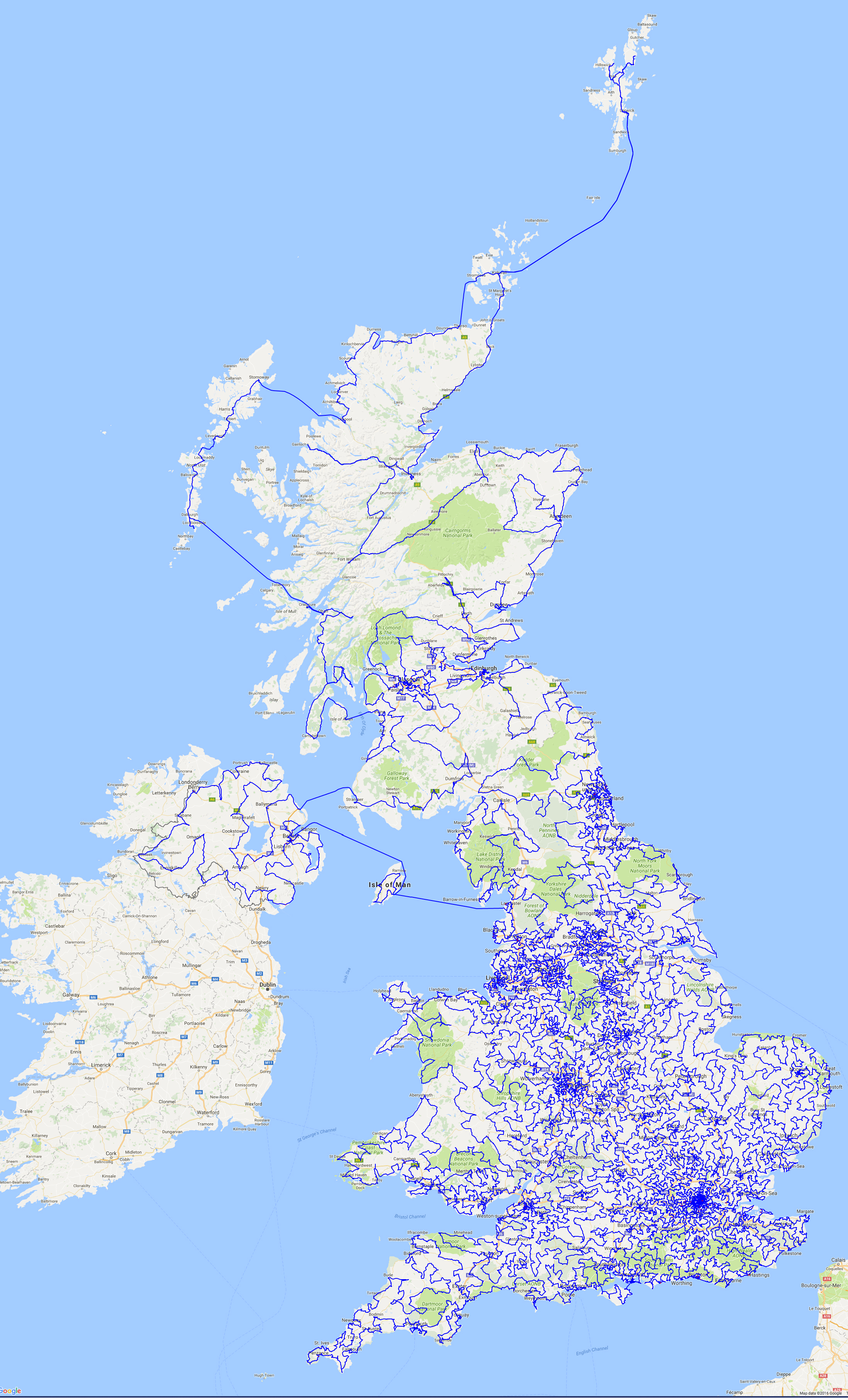
A walking tour of the UK’s pubs. A fine application of the Traveling Salesman Problem
Cheers!